Optimizing PyTorch Model Training: Balancing Speed and Memory Efficiency
Beyond Eager Mode: Advanced Memory Management for Deep Learning
PyTorch has become a cornerstone in deep learning development, offering flexibility and ease of use for researchers and engineers. However, as models grow larger and more complex, managing memory consumption while maintaining training speed becomes increasingly challenging. This blog post explores several techniques to optimize the trade-off between memory usage and computational speed during model training in PyTorch.
Understanding Eager Execution in PyTorch
Eager execution represents the default execution mode in PyTorch, where operations are executed immediately as they are encountered in the code. This offers great flexibility and intuitive debugging, making it popular among researchers and developers. In eager mode, when you call a function that uses the GPU, operations are enqueued to the particular device but not necessarily executed until later, allowing for parallel computation across CPUs or GPUs2. The framework executes one operation at a time, which provides a straightforward execution flow but can lead to significant memory consumption for large models.
During eager execution, tensors cannot reside on different devices (such as HPU and CPU) without explicit movement of one tensor to the HPU for efficient computation1. This immediate execution pattern means that each operation in your neural network consumes memory as soon as it's executed, which can quickly accumulate during training of complex models. The memory usage becomes particularly problematic when we store activations from the forward pass that are needed later for gradient computation during the backward pass.
Eager mode offers unparalleled flexibility and a pythonic look and feel that developers appreciate, allowing them to experiment with ideas without constraints. This is why it remains the default execution mode in PyTorch despite its memory inefficiencies. However, as we'll explore throughout this blog, there are numerous techniques available to optimize memory usage while preserving much of the convenience that makes PyTorch so attractive.
Activation Checkpointing: Trading Computation for Memory
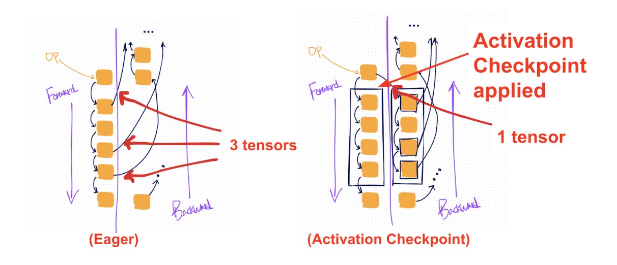
Activation checkpointing (also known as gradient checkpointing) represents a powerful technique to reduce memory usage during training by trading computational time for memory savings. This approach is particularly valuable when working with large models that would otherwise exceed available GPU memory. The fundamental concept behind activation checkpointing is straightforward: instead of storing all intermediate activations during the forward pass, we strategically save only a subset and recompute the others when needed during the backward pass.
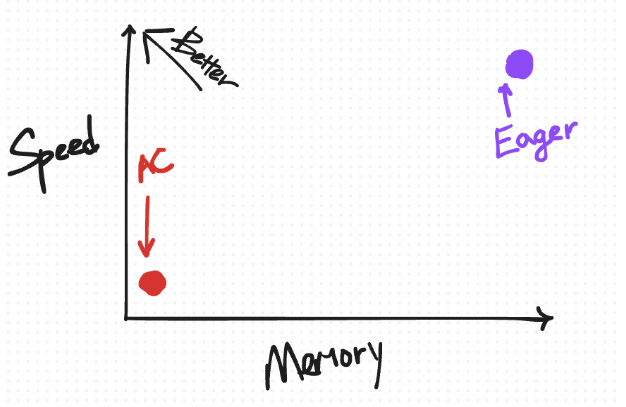
In traditional eager execution, every intermediate activation from the forward pass must be stored to compute gradients during backpropagation, resulting in substantial memory consumption that scales with model depth. By contrast, activation checkpointing allows us to discard certain activations after they're used in the forward pass, then recompute them during the backward pass when they're needed for gradient computation. This approach significantly reduces peak memory usage at the cost of additional computation, essentially trading GPU cycles for memory space.
Implementing activation checkpointing in PyTorch is relatively straightforward using the torch.utils.checkpoint module. When applied to specific model components, it can dramatically reduce memory consumption, often enabling training of models that would otherwise be impossible given available hardware constraints. The memory savings from activation checkpointing can be substantial, sometimes reducing memory requirements by 50% or more, though this comes at the cost of roughly 30% increased computation time due to the recomputation of activations.
Torch.compile and Min-cut Partitioner: Advancing Beyond Basic Checkpointing
The torch.compile feature introduced in PyTorch 2.0 represents a significant advancement in training optimization. Unlike eager mode where operators are dispatched individually, compile mode pre-compiles the entire model into a single optimized graph specifically tailored for the target hardware platform7. This approach not only improves performance but also enables sophisticated memory optimization techniques like min-cut partitioning.
When using torch.compile, the system traces both forward and backward pass computations into a single joint computational graph. This comprehensive graph is then processed by the min-cut partitioner, which applies a min-cut/max-flow algorithm to intelligently split the graph in a way that minimizes the number of tensors that need to be saved for the backward pass. The algorithm analyzes the entire computational flow and determines optimal checkpointing boundaries that balance memory usage and recomputation costs.
The partitioner primarily focuses on reducing runtime while managing memory constraints. It selectively chooses which operations to recompute based on their computational intensity and fusion potential. Typically, simpler, fusible, and non-compute-intensive operations (like pointwise operations) are candidates for recomputation, while more expensive operations might be preserved. This selective approach offers significant advantages over basic activation checkpointing, which treats all operations within a checkpointed region equally regardless of their computational cost.
The improvements from torch.compile can be substantial, with users reporting up to 2x better performance for Hugging Face model inference and up to 1.35x better performance for TorchBench model inference compared to default eager mode across various natural language processing, computer vision, and recommendation models7. These gains demonstrate how sophisticated compilation strategies can significantly enhance both memory efficiency and computational speed.
Selective Activation Checkpoint: Fine-grained Memory Management
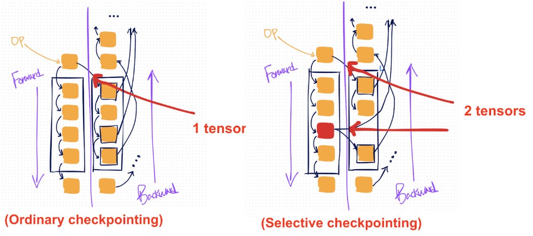
Selective Activation Checkpoint (SAC) represents an evolution of standard activation checkpointing by providing more granular control over which specific operations to recompute. While normal checkpointing recomputes every operation in the chosen region, SAC allows developers to selectively designate which operations should be saved and which should be recomputed, enabling more nuanced memory-computation trade-offs.
The key advantage of SAC lies in its ability to differentiate between expensive and inexpensive operations. Compute-intensive operations like matrix multiplications (matmul) consume significant GPU resources when recomputed, whereas simpler pointwise operations can be recomputed with minimal overhead. By selectively saving the results of expensive operations while recomputing cheaper ones, SAC achieves better overall performance than standard checkpointing for many models.
Implementing SAC in PyTorch involves defining a policy function that specifies which operations should be saved and which should be recomputed. For instance, a common policy might be to avoid recomputing matrix multiplication operations while allowing recomputation of simpler operations. This can be achieved by creating a policy function that returns CheckpointPolicy.MUST_SAVE for compute-intensive operations and CheckpointPolicy.PREFER_RECOMPUTE for others.
More aggressive policies might extend this approach to save a wider range of compute-intensive operations, including convolutions, flash attention operations, and other expensive computations. The choice of policy depends on the specific model architecture and available computational resources, allowing for customized optimization that maximizes performance within given memory constraints.
Implementing Selective Activation Checkpoint
Implementing SAC in your PyTorch code is relatively straightforward using the existing checkpoint API with additional context parameters. The implementation involves creating a policy function that designates which operations should be saved versus recomputed, then passing this function to the checkpoint API through the context_fn argument.
The policy function examines each operation and determines whether it should be saved or recomputed based on its type and computational intensity. For matrix multiplication operations, which are typically expensive to recompute, the policy might return CheckpointPolicy.MUST_SAVE to ensure these results are preserved. Conversely, for lightweight operations like activations and element-wise functions, the policy would return CheckpointPolicy.PREFER_RECOMPUTE to trade computation for memory savings.
To apply this in practice, you would first identify the compute-intensive operations in your model that should be saved rather than recomputed. These typically include matrix multiplications, convolutions, attention mechanisms, and other operations with high computational complexity. Once identified, you create a policy function that checks each operation against this list and returns the appropriate checkpoint policy.
This approach offers remarkable flexibility, allowing developers to fine-tune memory-speed trade-offs according to their specific requirements. By selectively choosing which operations to recompute, you can optimize performance within given memory constraints far more effectively than with standard checkpointing techniques that treat all operations equally.
Memory Budget API: Automating Optimization Decisions
Finding the optimal balance between memory usage and computational speed often requires extensive experimentation with different checkpointing policies. To streamline this process, PyTorch provides a Memory Budget API specifically designed for compiled models. This API automates the decision-making process regarding which operations to save versus recompute based on a specified memory budget.
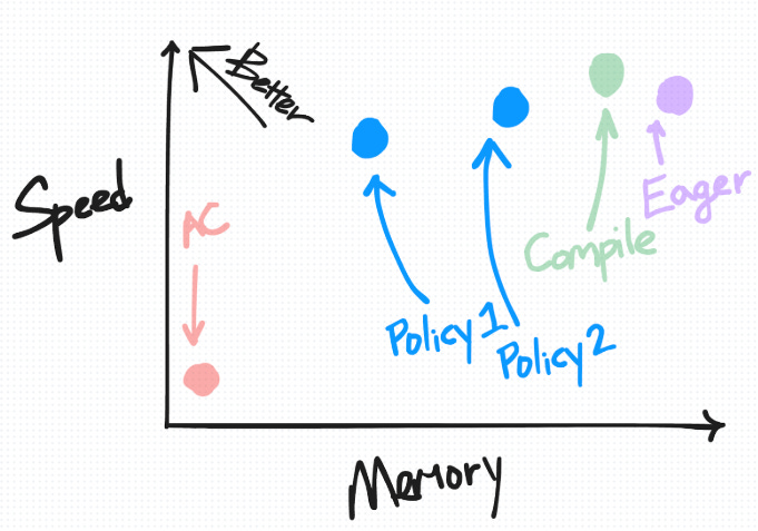
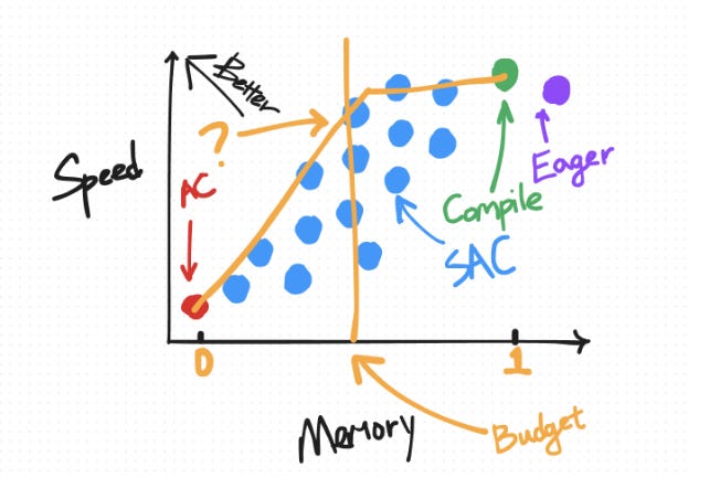
The Memory Budget API works with the observation that optimal policies tend to fall on what's known as a Pareto curve, representing the best possible trade-offs between memory usage and computational speed. Rather than manually testing various policies, developers can simply specify a memory budget parameter between 0 and 1, where 0 behaves like plain activation checkpointing (maximizing memory savings) and 1 behaves like default torch.compile (maximizing speed).
Using this API is remarkably simple; you set a memory budget parameter through the configuration option torch._dynamo.config.activation_memory_budget and then apply torch.compile to your function. The system automatically determines which operations to save and which to recompute to achieve the specified memory-speed trade-off. For example, setting the memory budget to 0.5 would aim for a balanced approach that provides moderate memory savings while limiting the performance impact.
This automated approach significantly simplifies the optimization process, especially for complex models where manually determining the optimal checkpointing strategy would be prohibitively time-consuming. However, it's important to note that this feature requires using compiled models through torch.compile, as it relies on the ability to analyze and optimize the full computational graph.
Conclusion: Selecting the Right Approach for Your Needs
Activation checkpointing techniques in PyTorch offer a versatile toolkit for balancing memory and computational demands during model training. From basic region-based checkpointing to sophisticated selective and automated methods, these approaches provide flexible solutions to address the memory constraints that often limit deep learning research and development.
The choice of optimization technique depends largely on your specific requirements and constraints. For simpler models or development scenarios where flexibility is paramount, eager execution remains an excellent default choice. When memory becomes a limiting factor, basic activation checkpointing provides a straightforward solution with minimal code changes. For more complex models where performance optimization is critical, selective activation checkpointing or torch.compile with the Memory Budget API offer more sophisticated approaches that can achieve better memory-speed trade-offs.
Understanding the performance characteristics of each technique allows you to make informed decisions based on your model architecture and available resources. By strategically applying these optimizations, you can train larger, more complex models without requiring expensive hardware upgrades, ultimately enabling more ambitious deep learning research and applications on existing infrastructure.
Frequently Asked Questions
What's the difference between activation checkpointing and gradient checkpointing?
Activation checkpointing and gradient checkpointing refer to the same memory optimization strategy in neural network training. Both terms describe the technique of trading computation time for reduced memory usage by selectively storing activations and recomputing them when needed for gradient calculation. The terminology difference mainly stems from different research communities and frameworks, but they fundamentally describe the same optimization approach where intermediate activations are discarded and recomputed to save memory during backpropagation.
How do activations and gradients relate to each other in memory-optimized training?
Activations and gradients are closely related in the context of memory-optimized training techniques like checkpointing. Activations are the intermediate outputs produced during the forward pass as data flows through the network from input to output. These activations are normally stored in memory because they're required later for computing gradients during the backward pass. Gradients, on the other hand, represent the rate of change of the loss with respect to model parameters, computed during the backward pass to guide parameter updates.
The relationship between activations and gradients creates the memory challenge that checkpointing addresses. During standard training, activations from the forward pass must be kept in memory until the corresponding gradient computation in the backward pass is complete. Checkpointing techniques strategically discard certain activations after the forward pass and recompute them during the backward pass when needed for gradient calculation, thereby reducing peak memory usage at the cost of additional computation time.
What exactly is eager mode in PyTorch?
Eager mode in PyTorch refers to the default execution mode where operations are executed immediately as they are encountered in the code rather than being compiled into a static graph first. In eager mode, when you perform an operation on a tensor, that operation is executed right away, and the result is returned immediately, providing a dynamic and intuitive programming experience7. This execution mode offers great flexibility for development and debugging, as variables can be inspected at any point, control flow statements work naturally, and code behaves much like standard Python.
While eager mode provides excellent usability and flexibility, it sometimes comes with performance trade-offs compared to graph-based execution modes. Operations executed eagerly may not benefit from certain optimizations that would be possible with a compiled approach, leading to potential inefficiencies in memory usage and computation time for complex models. This is why PyTorch has introduced features like torch.compile that can provide the benefits of graph-based optimization while maintaining much of the flexibility of eager execution.


